Manual LoRa Demodulation Given Limited Information
Demodulating LoRa manually is a non-trivial task that requires a deep and fundamental understanding of RF and LoRa. Although there exist plenty of tools on the Internet today that can easily and automatically demodulate LoRa given I/Q data and the right arguments, having limited information to inform the latter leaves a radio hacker with few choices besides embarking on manual LoRa demodulation.
Not only will this post cover manual LoRa demodulation in detail, but this post will also cover the background and fundamentals. The goal is to equip a novice, someone with no prior radio hacking experience and only basic trigonometry skills, with the knowledge and confidence to embark on this non-trivial task.
NOTE: this post is still being authored, and this is just a preview.
Background
Radio
“RF is easy. It’s all just spicy sines.”
- Shawn “skat” Kathleen
Radio refers to a subset of the electromagnetic spectrum spanning between 3 Hz and 300 GHz in frequency, called radio frequency (RF). These electromagnetic waves, called radio waves, are commonly used for wireless communications. When we change one or more properties about these radio waves, we can transmit data; this is a process known as modulation: the variation of one or more properties of a periodic waveform (a carrier signal) with a data signal (modulation signal) in order to transmit data over radio waves.
Although “RF” stands for radio frequency, it colloquially refers to the subject of radio more broadly.
In a basic radio communications scenario, there are two actors: the transmitting party, and the receiving party. Both parties are equipped with an antenna. The transmitting party applies current to the transmitting antenna which radiates radio waves into space, and the receiving party has a receiving antenna that absorbs some of the radiated power in order to produce a current. That is to say, the transmitting party sent a radio wave to the receiving party.
In a basic scenario, the transmitting party may be emitting a simple periodic waveform: a sinusoid. Recall that the general form for a sinusoid is:
\[\begin{align} y(t) = A\,sin(\omega t + \phi) \end{align}\]where
- \(A\) is the amplitude;
- \(\omega\) is the angular frequency in radians per second;
- \(t\) is time in seconds; and
- \(\phi\) is the phase shift in radians.
Recall that angular frequency, \(\omega\), is related to ordinary frequency by \(\omega = 2\pi f\).
Although “sine” refers to the trigonometric sine function, a “sinusoid” refers to a sine wave of arbitrary parameters. Colloquially, people may refer to “sinusoids” as “sines.”
A basic sinusoid may look like this:
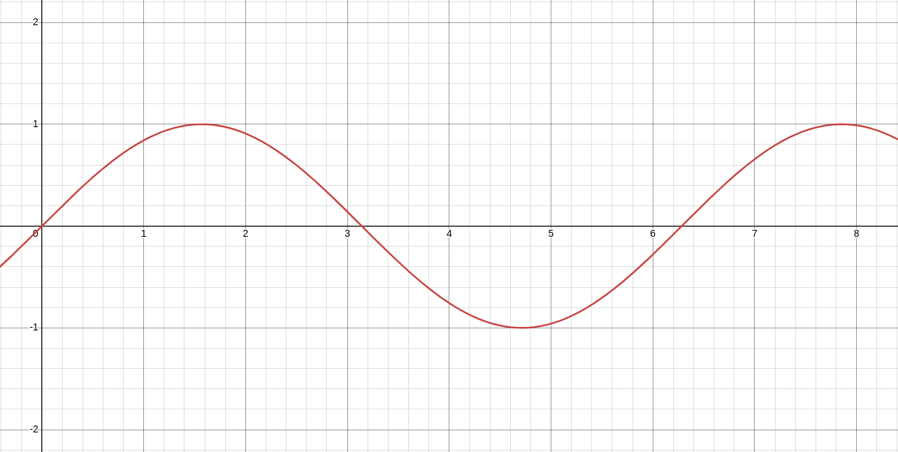
Since we’re talking about radio frequency, the frequency should be higher than the sinusoid shown above. For example’s sake, I’ll be using the lower bound of the range of radio frequency: 3 Hz, which is considered extremely low frequency. Keep in mind that real-life radio applications are commonly 125 kHz, 13.56 MHz, 433 MHz, 918 MHz, 2.4 GHz, 5 GHz, and more. 3 Hz is great for an example, but uncommon in reality.
Note that the amplitude did not change. Pay attention to the axes and scaling, as that will be relevant throughout this section.
The transmitting party sent a 3 Hz sinusoid to the receiving party. The receiving party received the signal, and now they have the transmitting party’s 3 Hz sinusoid. There’s not much information to be gained besides the presence of a radio wave and the frequency thereof. For some applications, this may be fine; consider a basic alarm that goes off when a radio transmission on a certain frequency is detected.
Since a transmitting party can also stop transmitting, this enables the transmitting party to send another important piece of information: the duration of a transmission. By encoding data into variable-duration transmissions, we can at minimum develop a binary information system to transmit data. One of the earliest and most well-known examples of this is Morse code, where an alphanumeric character set is encoded into dots and dashes – short and long transmissions. The idea of changing something in order to send information is essential to radio communications, both in the digital and analog realms.
Recall that modulation is the variation of one or more properties of a periodic waveform (a carrier signal) with a data signal (modulation signal) in order to transmit data over radio waves. In the case of radio transmissions, the carrier signal is almost always analog, though the data signal may or may not be. As a sinusoid, the modifiable properties of a carrier signal are the modifiable properties of a sinusoid: the amplitude (\(A\)), frequency (\(f\)), and phase shift (\(\phi\)). With an analog data signal, this results in amplitude modulation (AM), frequency modulation (FM), and phase modulation (PM), respectively. With a digital data signal, this results in amplitude-shift keying (ASK), frequency-shift keying (FSK), and phase-shift keying (PSK), respectively.
In the digital realm, there are many more modulation schemes exist than just ASK, FSK, and PSK, including a special scheme that we’ll discuss later that explores the idea of “chirping.”
Suppose that we want to transmit the bits “0110” using ASK, FSK, and PSK in order to see what it’d look like. With ASK, we can let \(A_0\) and \(A_1\) be any two different values, such as \(0\) and \(1\):
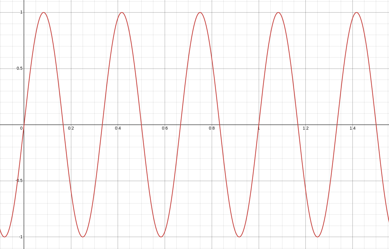
With FSK, we can let \(f_0\) and \(f_1\) be any two different values, such as \(3\) and \(6\):
With PSK, we can let \(\phi_0\) and \(\phi_1\) be any two different values from \(0\) to \(2\pi\), such as \(0\) and \(\pi\):
In PSK, you’re limited from \(0\) to \(2\pi\) because a phase shift of \(2\pi\) is equal to a phase shift of \(0\).
To put concisely, radio signals are a subset of electromagnetic signals operating within the radio frequency range, and we can modify one or more properties of a carrier signal in conjunction with a data signal through a process known as modulation in order to embed data in radio waves propagating through space. This enables us to transmit data wirelessly, unlocking wireless communications.
This is cool and all, but in the real world, we run into a few important issues that hamper the effectiveness of radio transmissions.
Propagation Complications
There are a variety of complications that make propagation more nuanced in the real world. Electromagnetic waves propagating through free space lose intensity as a function of distance dictated by the inverse square law due to wave spread. These waves may additionally collide with obstacles, be reflected, take multiple paths to arrive at a destination, or interfere with themselves or with other waves, among a long list of other factors. We can usually make assumptions and simplify variables in order to arrive at radio propagation models, but these are imperfect and just approximations; as it turns out, it’s pretty difficult to accurately account for every single complication in radio propagation.
An example of a widely used radio propagation model is free-space path loss (FSPL), which only accounts for the loss of signal intensity between two antennas as a function of distance, not taking into account any other factors like reflection, refraction, or absorption.
\[\begin{align} \frac{P_r}{P_t} = D_t D_r \left(\frac{\lambda}{4\pi d}\right)^2 \end{align}\]where
- \(P\) are the powers received (\(r\)) and transmitted (\(t\));
- \(D\) are the directivity of the receiving (\(r\)) and transmitting (\(t\)) antennas, or 1 in the case of isotropic antennas;
- \(\lambda\) is the signal wavelength; and
- \(d\) is the distance between the antennas.
Because this is so simple and fundamental, this is one of the most commonly used models for radio propagation.
Unfortunately, we live in the real world, so we have to deal with the complications. Transmitting instruments can only output signals with so much power before being subject to the limitations of the physical environment, and receiving instruments can only make sense of received signals if they’re above the instrument’s minimum signal sensitivity threshold and are adequately uncorrupted. In the case that a signal is above a receiving instrument’s minimum signal sensitivity threshold, but has been corrupted due to any of the factors listed earlier, the transmitting party can make a sub-optimal link more feasible through error detection and correction codes.
Not all wireless links are feasible, and we can only effectively communicate if the link budget allows. If we’re not making the budget, we have to change one or more parameters of the scenario in order to meet the budget: increase transmission power, decrease distance, use more sensitive instruments, etc. each with their own pros and cons and cost-benefit and diminishing return curves.
Amongst the many things we could do, there exist a few techniques that can increase the budget in order to help us make a link feasible through the modulation schemes themselves. One such technique is something known as chirp spread spectrum.
It’s easy to think about just increasing transmission power, but your locale’s agencies governing radio frequency may have a thing or two to say. In the United States, the Federal Communications Commission (FCC) governs radio frequency and imposes limits on transmission power. In addition, many applications of radio – such as Internet of Things (IoT) or wireless sensor networks (WSNs) – may be constrained systems whose best interest is to conserve energy in favor of extended lifetimes. In either case, increasing transmission power generally carries diminishing returns due to the inverse square law, especially in the case of isotropic antennas.
Chirp Spread Spectrum (CSS)
Suppose that we had a modulation scheme where we changed the frequency, but not in a keyed way. That is to say, when sending a message that has \(n\) many symbols, we don’t simply modulate by discretely switching between \(f_0\), \(f_1\), … \(f_{n-1}\) in order to encode the symbols. Instead, suppose that we modulate symbols by increasing or decreasing frequency as a function of time. This is a concept known as “chirping,” where a function of time allows us to sweep a frequency range.
Sweeping a frequency range offers a variety of benefits that can increase our link budget. In particular, we gain resiliency against channel noise, interference, and multi-path fading. This allows a recipient to detect and demodulate the signal with greater success in the presence of noise and interference, effectively improving the link margin. Unfortunately, this comes with the cost of a drastically reduced data rate.
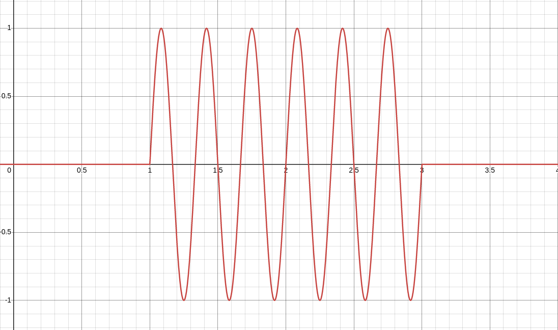
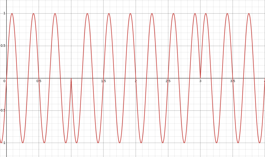
As a very basic example, suppose that we let \(f_0(t') = nt'\) and \(f_1(t') = -nt'\), where \(t'\) is time since the start of the chirp and \(n\) is the difference between our upper and lower frequency bounds. For example’s sake, let’s change from 3 Hz and 6 Hz to 300 Hz and 600 Hz in order to take advantage of the benefits of CSS.
Occupying a frequency range from 300 Hz to 600 Hz, this means that instead of “0” and “1” symbols being 300 Hz and 600 Hz sinusoids sent for fixed durations of time, respectively, a “0” symbol is the increase from 300 Hz to 600 Hz and a “1” symbol is the decrease from 600 Hz to 300 Hz, each at a linear rate of 300 Hz per second.
These functions and numbers were chosen for example’s sake. You can have different frequencies. You can even have non-linear functions dictate the rate at which a frequency range is swept.
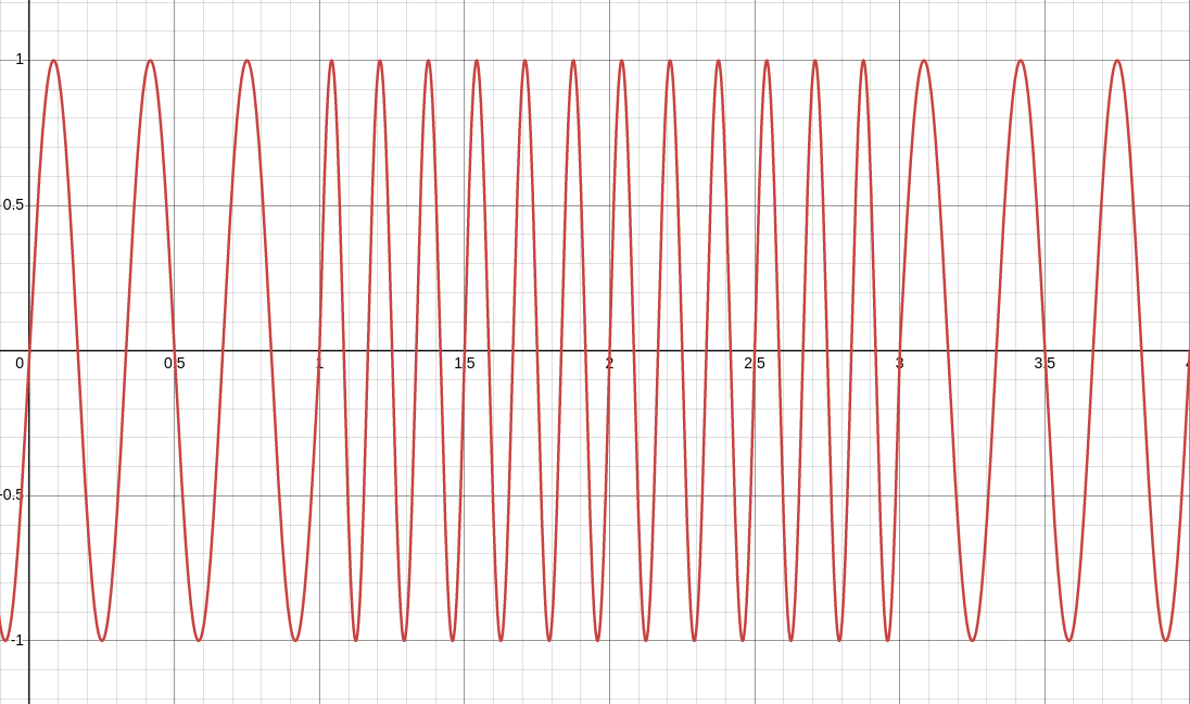
When working with frequency modulation techniques, as we saw with FSK, this can be difficult to visually see when we inspect amplitude over time. Here’s just one section of a chirp:
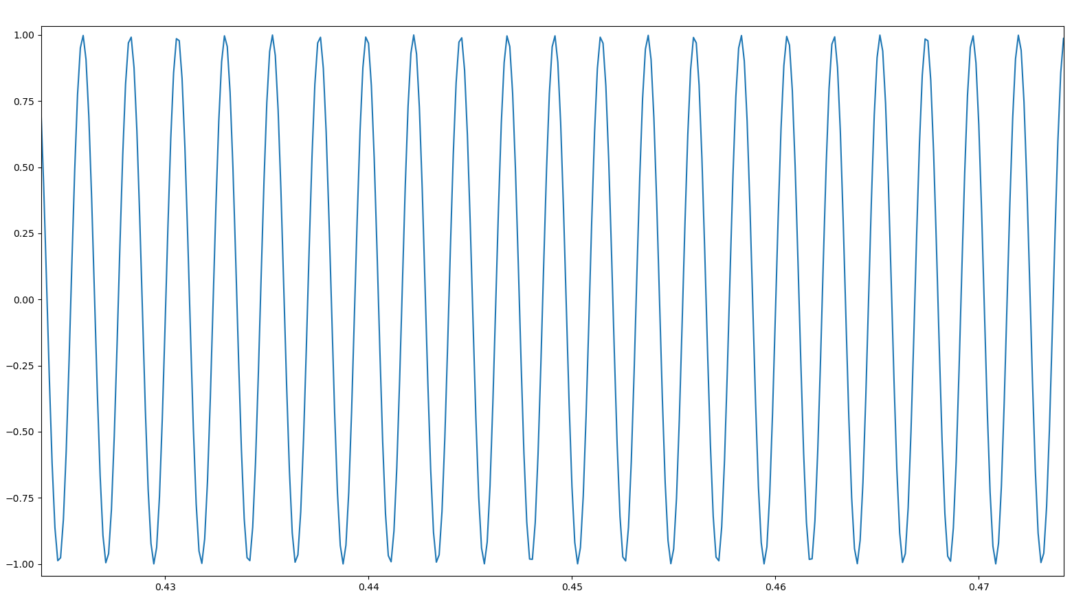
Is the frequency increasing or decreasing? What is the rate at which it’s changing? These questions aren’t easy to answer – yet. We need some more things to add to our toolbox in order to gain a sufficient enough understanding to move forward.
Fourier Transforms and FFTs
The Fourier transform is a tool that allows us to take a function of time and turn it into a function describing its constituent frequencies. This post won’t go too in-depth into the inner workings of Fourier transforms since it’s a bit mathematically dense and requires some calculus, and this post stated earlier that the target audience is a novice with only basic trigonometry skills. However, broadly understanding the purpose and usage of this tool is important for beginners.
To quickly visualize what Fourier transforms allow us to do:
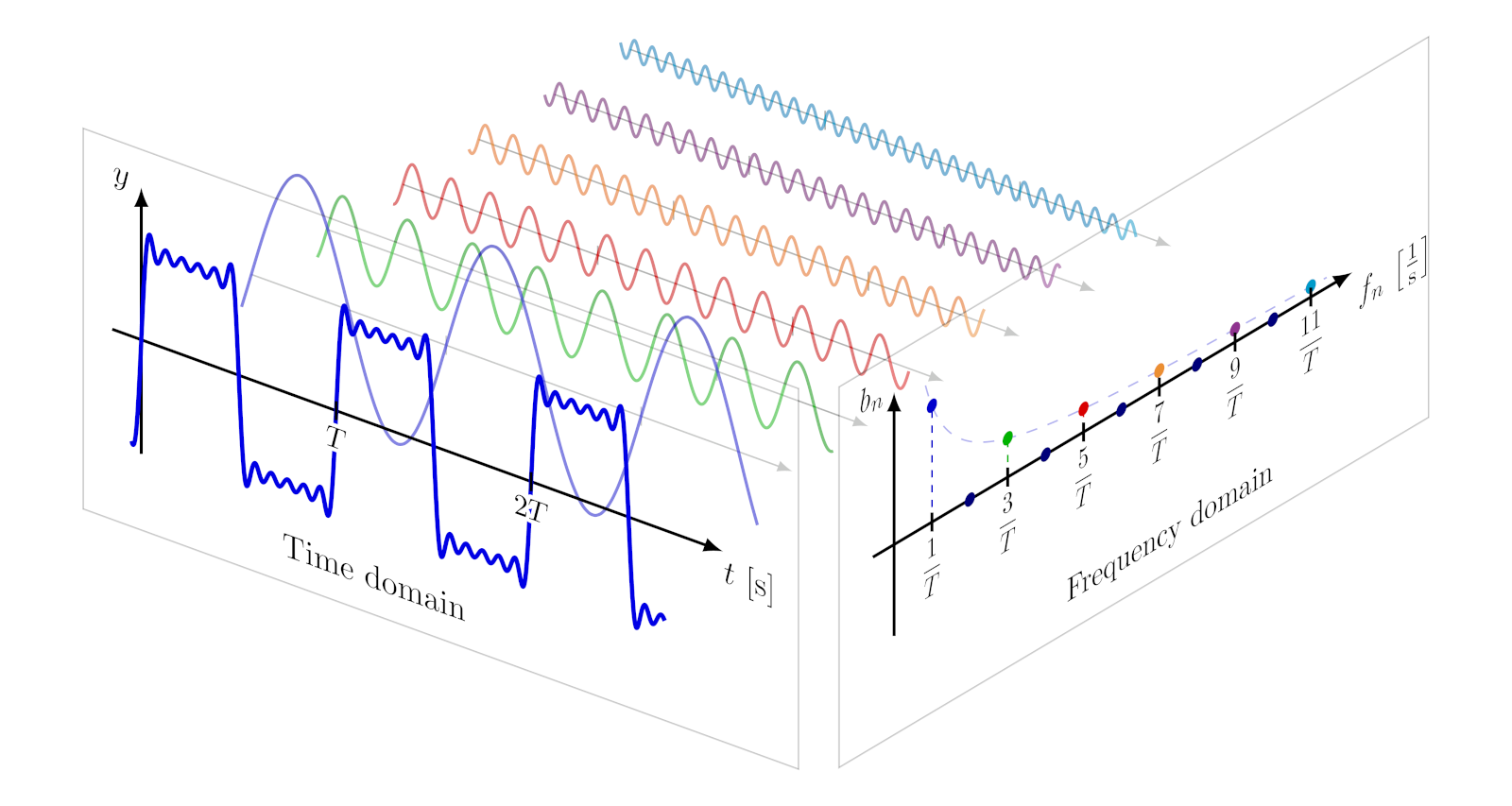 Credits to Izaak Neutelings, CC BY-SA 4.0. TikZ contains great visuals. All I did was add a white background for visibility on this blog.
If you want to learn more about Fourier transforms in greater detail, 3Blue1Brown has an excellent introductory video:
Fourier transforms are an essential tool for radio, but a deep understanding of the underlying math is not necessary for beginners.
There are some reasons why Fourier transforms don’t work out-of-the-box for practical radio hacking. When dealing with real-life digital radio systems, received analog signals are converted into digital signals using analog-to-digital converters (ADCs), who have finite resolutions. We have to work with samples constrained by the sampling rate. Working in the digital space offers us many advantages, but we must understand that we sacrifice pure, analog precision as a trade-off.
Did you notice how the sines in the “Chirp Spread Spectrum (CSS)” section were jagged? Have you ever tried zooming in on a capture sample in a tool like Universal Radio Hacker (URH) and seen jagged edges?
I sometimes call these “crunchy sines.” Not a technical term.
A fundamental theorem in digital signal processing (DSP) is the Nyquist-Shannon Sampling Theorem, which states that the sample rate of an analog signal must be at least twice the bandwidth of the signal in order to avoid aliasing. That is to say, radio hackers must use at least twice a signal’s bandwidth as the sample rate when capturing signals in order to avoid loss of information due to insufficient resolution. If capturing with a 2 MHz bandwidth, your sample rate must be at least 4 MHz.
Assuming that we’ve met the Nyquist rate, we now have a viable finite sequence of discrete sample points, but we still have the problem of Fourier transforms operating on continuous data; our discrete data will not suffice.
Luckily, we have another tool available to us: the discrete Fourier transform (DFT). As you can probably tell from the name, the discrete Fourier transform is able to turn a finite sequence of time-domain samples into the corresponding sequence of frequency-domain components. Just like normal Fourier transforms, this allows us to analyze a signal’s frequency contents. DFTs are useful in the digital space, though a deep understanding of their inner workings are not necessary for beginner radio hackers.
One of the issues of DFTs is that they can be slow, with a time complexity of \(O(n^2)\). Enter yet another tool: the fast Fourier transform (FFT). FFTs are easily one of the most important sets of algorithms for RF and DSP. FFTs are able to reduce the computational complexity from \(O(n^2)\) to \(O(n\,log\,n)\). This is massive and opens the door to the practicality of many applications of Fourier transforms in the digital space.
When we plot FFTs over time, we can create spectrograms. Spectrograms allow us to visualize the frequency spectrum of a signal over time. If you’re ever scanning the air to see what’s going on, this allows you to see what frequency channels are in use. If you’re using CSS, this allows you to visually see the sweep of a chirp:
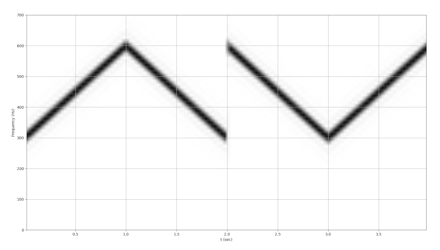
With upchirps being 0 and downchirps being 1, this just says “0110” using a very basic CSS modulation scheme.
NOTE: this post is still being authored, and this is just a preview. LoRa section is currently under review for accuracy and GRC section is still being planned.
History
- 2024.05.23: Initial post as a preview.
- 2024.06.06: Published “Propagation Complications” and “Chirp Spread Spectrum (CSS)” sections.
- 2024.06.13: Published “Fourier Transforms and FFTs” section.
- 2024.06.16: Grammatical/stylistic edits and revisions.
- (Planned): “GRC and LoRa” sections.